Section 1: Introduction and Descriptive Statistics
Section 1.1: Getting Access to Stata
Section 1.2: Displaying Data
This part shows you the general structure of Stata command, we will start learning Stata by loading Stata-format data (*.dta file) and simply display the data at hand.
Getting an overview of your file
The sysuse command can load a specific .dta file provided by Stata itself.
sysuse auto.dta
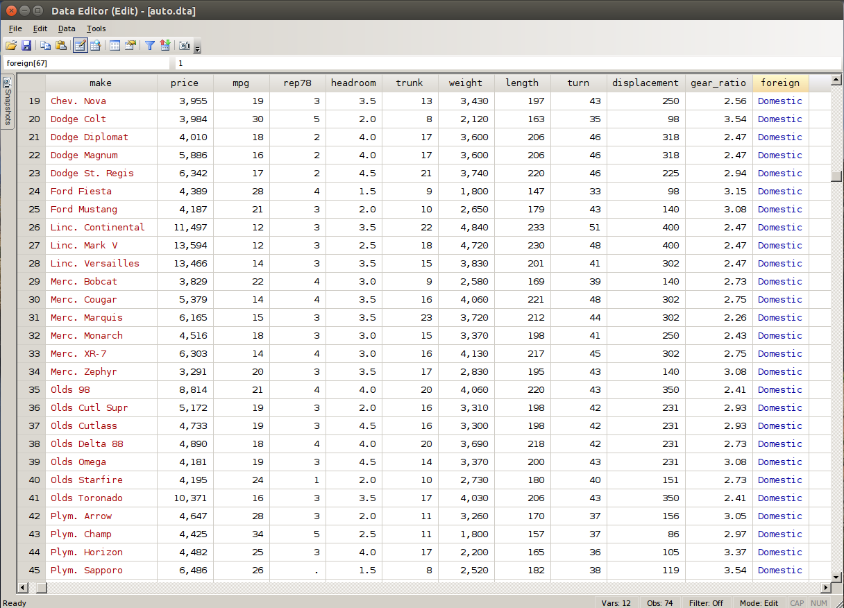
The edit command can provide an Excel alike view of your data file. And this is how the file auto.dta looks like after invoking edit command.
edit
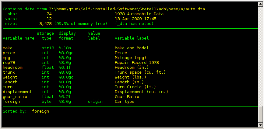
The describe command shows you basic information about a Stata data file. As you can see, it tells us the number of observations in the file, the number of variables, the names of the variables, and more.
describe
The output from Stata is here
Displaying Nominal(Categorical) Variable
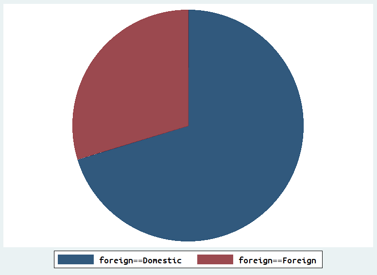
We use the variable “foreign” in auto.dta to demonstrate how to generate pie chart and bar chart for this nominal variable.
In Stata, pie and bar charts are drawn using the sum of the variables specified. Here variable “foreign” contains labeled integers (0 or 1), command tabulate can be used to show counts or frequencies of those integer values. To create pie charts, first run the variable through tabulate to produce a set of indicator variables:
tabulate foreign, generate(f)
graph pie f1 f2
The pie chart is here
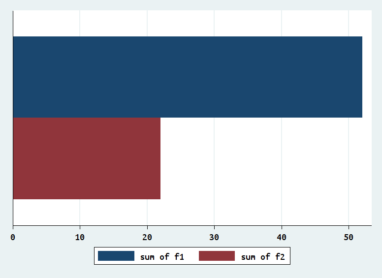
Bar chart can also be produced once variable f1 and f2 are generated:
graph hbar (sum) f1 f2
The bar chart is here
The tabulate foreign, generate(f) command generates two indicator variables f1 and f2, you may use drop command to delete this two variables so as to get back to our original data set.
drop f1 f2
Displaying Interval Variable
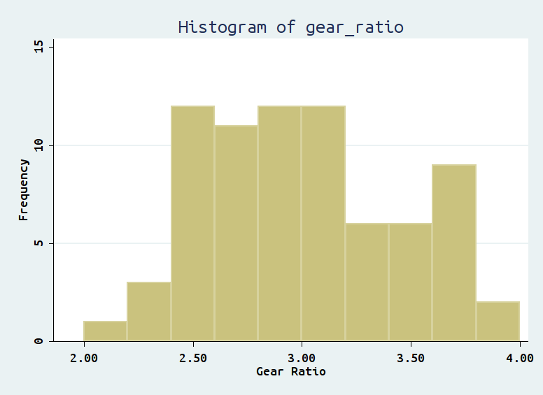
Histogram can provide the visual display of an interval variable without including all the individual values of this variable. The histogram command can fulfill this task.
histogram gear_ratio, width(.2) start(2.0) frequency title("Histogram of gear_ratio")
The above command is a good example to demonstrate the structure of commands in Stata. The part before comma is the core command, telling Stata what to do. In our case, histogram gear_ratio tells Stata to generate a histogram for the variable “gear_ratio”; the part after comma gives additional options to the core command, telling Stata ways to refine the histogram. The first two options indicate the width of histogram should be .2 and the lower bound of first bin of histogram should be 2. Option “frequency” tells Stata y axis of the histogram should be frequencies, the default value is “density”. Option “title” should be intuitive, asking Stata to add a title to the histogram. In order to familiarize yourself with the way Stata command works, you could add all the above options one by one to see how each of those options change the way histogram looks.
Finally, the output should be shown as follows.
Section 1.3: Central Tendency and Variability
In this section, let’s create our own data and use self-created data set to get the information about central tendency and variability of the data.
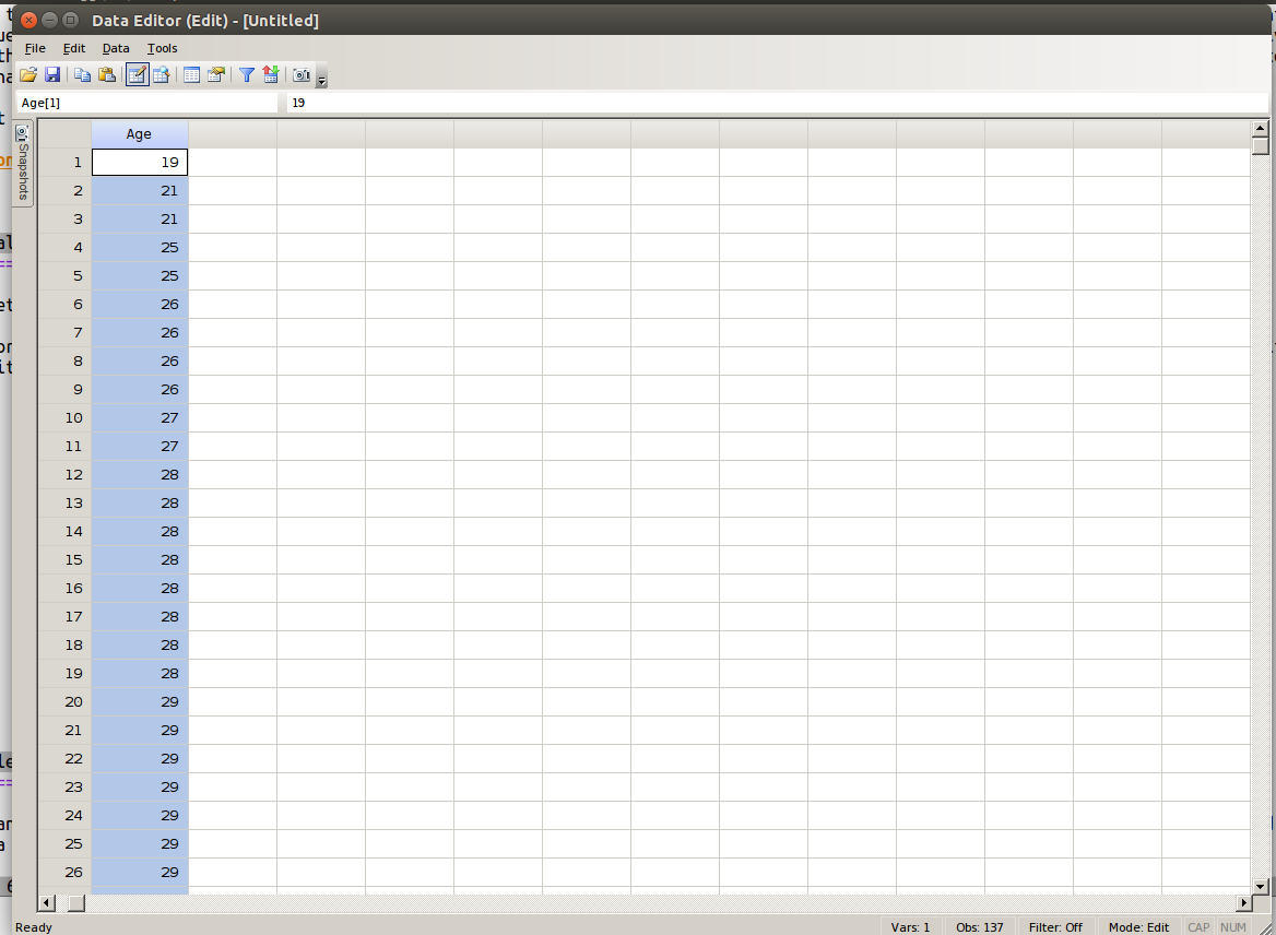
The most straightforward way to create your own data is to use data editor. You can simply type in the command edit or click the “Data Editor (Edit)” button to invoke the data editor. Then in the pop-up window, you can input data the same way as you would in Excel.
To rename the variables (which are automatically named var1, var2, etc.), right click on one of the cells in the column you want to rename and then choose “Variable Properties” to change the name. If everything is done right, the data editor should look like the following window.
In order to use the data later, one needs to save it. By simply clicking “File->Save as...”, you can specify the name of the file (age.dta for instance) and the path you want to save the file.
To analyze the data age.dta we created, we need to tell Stata where to find the data file. One way to do this is go to “File->Change Working Directory...” to locate the path where age.dta is stored.
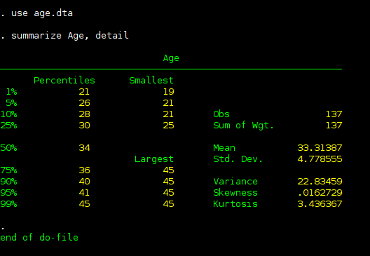
Then the following command can be used to find out the central tendency of the data age.dta.
use age.dta
summarize Age, detail
The output which can be found below displays the median (50% percentile), the mean, the standard deviation as well as other statistics.
Do-file
You can always organize your commands in do file. For the exercise we did above, you can find the do file below. You may want to download it and familiarize yourself with Stata commands we learned in this section.
Try to develop the habit of using do file at the beginning, you will find it extremely helpful in keeping track of your project.